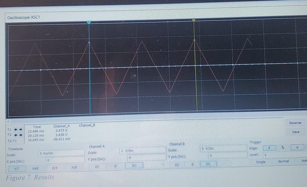
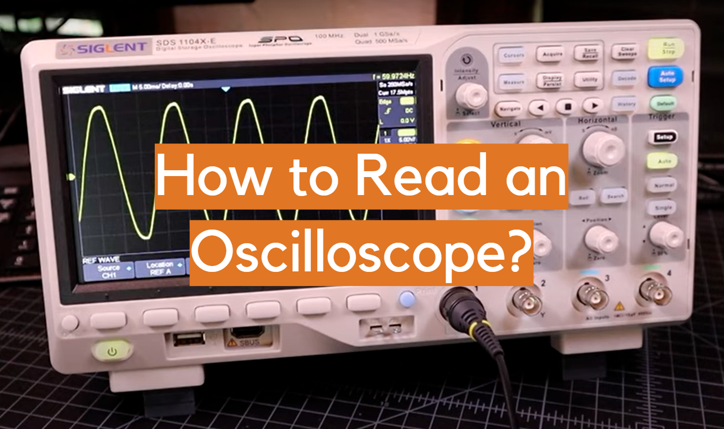
How to Master the XSC1 Oscilloscope: An Essential Guide
If you’ve just added an Oscilloscope XSC1 to your bench, you’re probably wondering where to start. This guide walks you through the basics—unboxing, core controls, signal capture, and a handful of tips that keep the instrument reliable day after day. By the end, you’ll feel confident tweaking the XSC1 for everything from simple sine‑waves to noisy digital pulses.
Why the XSC1 Stands Out
The XSC1 packs a surprisingly large bandwidth for its price class, often hovering around the 100 MHz mark, which makes it suitable for hobbyist projects and light‑industrial work alike. Its 7‑inch color display offers a clear view of waveforms without the eye‑strain that older monochrome units can cause. Moreover, the built‑in USB interface lets you save screenshots or export CSV data directly to a PC, a feature that many competing models still lack.
Getting Started: Unboxing and Setup
Inside the box you’ll find the main chassis, a power cord, a BNC cable, and a quick‑start sheet. After plugging the unit into a grounded outlet, power it on and let the self‑calibration routine finish—this usually takes under a minute. The first screen you’ll see is the default “Auto‑Setup” mode, which automatically adjusts vertical and horizontal scales based on the input signal.
Core Controls and What They Do
Understanding the front‑panel knobs is the next step. The vertical position knob slides the trace up and down, while the volts‑per‑division (V/div) dial changes the amplitude scaling. Horizontal time‑base controls the sweep speed, letting you zoom in on fast transients or view longer periods in a single sweep. A few buttons—Run/Stop, Single, and Auto‑Setup—handle basic acquisition without digging into menus.
Capturing and Analyzing Signals
To capture a waveform, connect the probe’s tip to the test point and the ground clip to a common reference. Set the probe attenuation (usually 1× or 10×) on the XSC1, matching the physical probe setting to avoid amplitude errors. Once the trace appears, you can press Measure to bring up common parameters: peak‑to‑peak voltage, frequency, and RMS value. For more detailed analysis, switch to the “FFT” mode, which transforms the time‑domain trace into a frequency spectrum—handy for spotting unwanted harmonics.
Practical Tips for Accurate Measurements
- Mind the Probe Bandwidth. A 100 MHz probe paired with a 100 MHz scope can introduce attenuation at the upper limit; consider a higher‑bandwidth probe for precise high‑frequency work.
- Use Proper Grounding. A loose ground lead can act like an antenna, injecting noise into the signal. Keep the ground clip short and attached close to the measurement point.
- Adjust Trigger Settings. A stable trigger prevents the trace from rolling across the screen. Start with “Auto” and then fine‑tune the level and slope for a crisp, stationary waveform.
- Save Frequently. The XSC1’s USB port makes it easy to archive screenshots or raw data; a quick “Save” before changing settings safeguards your work.
Common Issues and Quick Fixes
Even a well‑designed instrument can run into hiccups. If the display appears dim or washed out, check the brightness knob—some users inadvertently lower it while adjusting contrast. A “No Signal” warning often means the probe isn’t properly seated or the input coupling is set to DC when AC is needed. When the unit refuses to power on, verify that the mains voltage matches the rating on the back panel; the XSC1 typically expects 100‑240 V, so a mismatched adapter can cause a protective shut‑down.
Extending the XSC1’s Capabilities
Beyond the built‑in functions, the XSC1 supports firmware upgrades via the USB port. Periodically checking the manufacturer’s website ensures you have the latest bug fixes and feature additions—sometimes new analysis tools are added without requiring new hardware. Additionally, many users pair the scope with open‑source software like Sigrok to gain advanced decoding options for serial protocols, turning a modest bench instrument into a versatile debugging companion.
FAQ
Q: Can the XSC1 measure true RMS voltage for non‑sine waves?
A: Yes, the “Measure” menu includes a true RMS option, though accuracy depends on the probe’s bandwidth and proper calibration.
Q: How do I reduce aliasing when sampling fast signals?
A: Lower the time‑base to increase the sampling rate, and consider using the built‑in anti‑aliasing filter if the scope offers one.
Q: Is the XSC1 suitable for automotive diagnostics?
A: For low‑frequency sensor work and basic PWM analysis, it performs adequately. However, high‑frequency ECU signals may exceed its bandwidth, so a higher‑spec scope might be needed.
Q: What’s the best way to keep the XSC1 calibrated?
A: Run the auto‑calibration routine weekly, and store the unit in a dust‑free environment. For critical work, a professional calibration service once a year can verify the internal reference standards.