Mastering Refrigeration Cycle Calculations: A Step‑by‑Step Guide
Mastering refrigeration cycle calculations is essential for engineers, technicians, and students who design, troubleshoot, or maintain HVAC systems. This guide walks you through the core concepts, formulas, and practical steps that turn raw data into reliable performance predictions. Whether you’re working with a basic household refrigerator or a commercial chiller, the principles remain the same.
Understanding the Basics of the Refrigeration Cycle
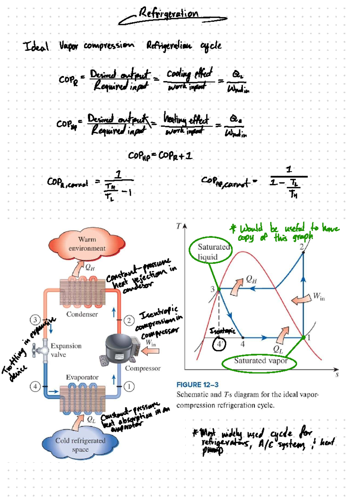
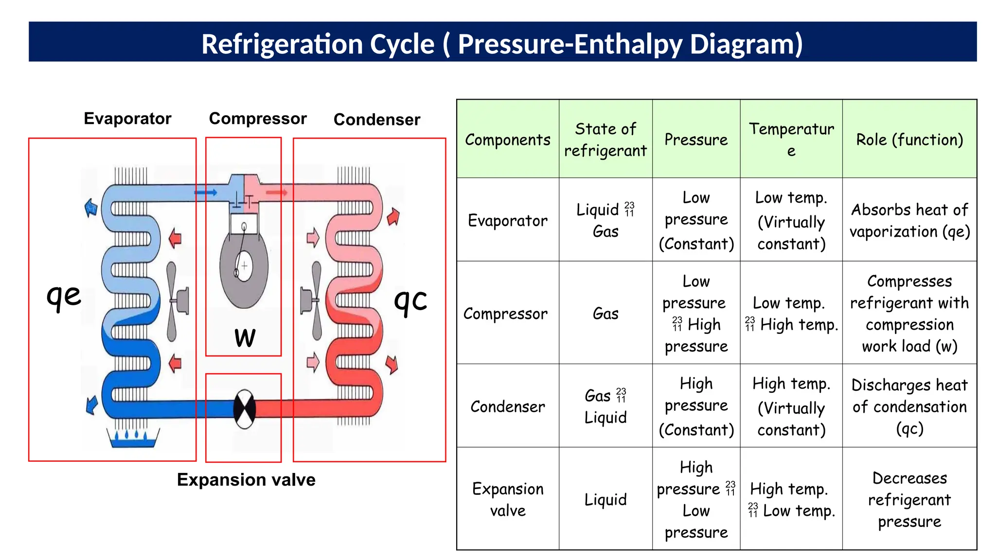
The vapor‑compression cycle, the backbone of most refrigeration systems, consists of four main components:
- Compressor – increases pressure and temperature.
- Condenser – releases heat to the surroundings.
- Expansion Device – drops pressure, causing partial evaporation.
- Evaporator – absorbs heat from the refrigerated space.
Each component corresponds to a state on a pressure‑enthalpy (p‑h) diagram, and the transition between states is governed by thermodynamic principles.
Key Thermodynamic Properties and Their Sources
Accurate calculations depend on reliable property data. Common sources include:
- Industrial tables and charts for saturated and superheated refrigerants.
- Commercial software like REFPROP or EES.
- Manufacturer data sheets for specific refrigerants.
Typical properties needed are enthalpy (h), temperature (T), pressure (p), and specific volume (v). Superheat and subcooling are critical corrections that account for non‑ideal behavior.
Step 1: Determine System Parameters and Refrigerant Choice
- Identify the working refrigerant – common examples include R22, R134a, and R410A.
- Set the evaporator and condenser operating conditions – typically expressed as pressure or temperature limits.
- Decide the mass flow rate (ṁ) – often derived from cooling load specifications.
Step 2: Calculate Compressor Work
The compressor raises the refrigerant from low to high pressure. Work per unit mass is:
Wc = (h2 – h1) / ηis
where ηis is the isentropic efficiency (typically 0.8–0.9 for small compressors). If ηis is unknown, assume 0.85 as a reasonable estimate.
Step 3: Compute Condenser Heat Rejection
Heat rejected in the condenser per unit mass is:
Qcond = ṁ × (h3 – h4)
Subtract any additional losses, such as fan power or piping friction, to get the net condenser duty.
Step 4: Find Evaporator Heat Absorption
Heat absorbed in the evaporator is:
Qevap = ṁ × (h1 – h4)
Ensure that the evaporator outlet temperature aligns with the required cooling load.
Step 5: Calculate Coefficient of Performance (COP)
The COP measures system efficiency:
COP = Qevap / Wc
Higher COP values indicate better energy utilization. Compare the calculated COP against industry standards or manufacturer claims to assess performance.
Common Pitfalls and How to Avoid Them
- Ignoring superheat and subcooling – neglecting these corrections can lead to under‑ or overestimation of duty cycles.
- Using incorrect refrigerant data – always cross‑check table values and software outputs.
- Assuming 100% compressor efficiency – unrealistic and will skew COP.
- Neglecting mechanical losses – fan, pump, and valve losses can add up.
Putting It All Together: A Sample Problem
Assume a R134a system with an evaporator



)