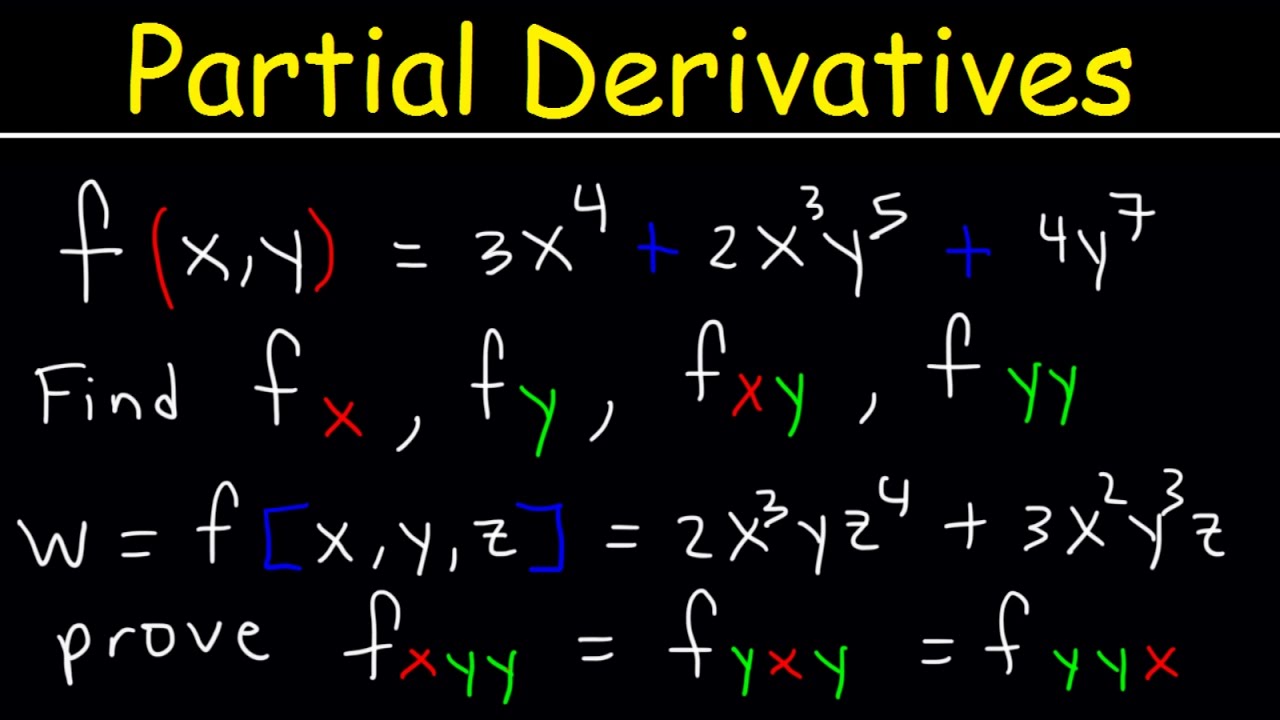
Partial Derivatives Explained: A Practical Guide For Beginners

If you’ve ever stared at a calculus textbook and felt your brain melt, you’re not alone. Partial derivatives often appear as the final boss of introductory multivariable calculus, intimidating with their Greek letters and multi-layered notation. But beneath the complex symbols lies a surprisingly intuitive concept. In fact, once you strip away the academic jargon, partial derivatives are just normal derivatives wearing a disguise.

Understanding them is crucial for anyone venturing into data science, physics, economics, or engineering. Whether you are trying to optimize a machine learning model or simply understand how temperature changes across a metal plate, partial derivatives provide the mathematical language to describe change in a multi-dimensional world.

Why One Variable Is No Longer Enough

To grasp partial derivatives, we first need to look at the standard derivative you likely learned in single-variable calculus. Traditionally, you deal with functions like $f(x) = x^2$. Here, $y$ depends entirely on $x$. If $x$ changes, $y$ changes in one specific direction. It’s a straight line or a smooth curve on a flat 2D graph. Calculating the slope here is straightforward: you draw a tangent line and measure its steepness.

But reality is rarely that simple. Consider a hill. Your elevation depends on both your north-south position and your east-west position. Mathematically, this is a function of two variables, perhaps $f(x, y) = z$. Now, if you take a step, your height changes, but which direction are you facing? Are you walking uphill along the ridge, or are you traversing sideways across the slope?

This is where the concept of "holding things constant" becomes your best friend. In the real world, everything is connected, but to analyze a complex system, we must isolate variables. Partial derivatives allow us to do exactly that. They measure how a function changes when you tweak one input while freezing all others in place.

The Core Concept: Freezing Variables

Imagine you are driving a car. Your fuel efficiency might depend on two things: your speed and the weight of the cargo. Let’s say you want to know how fuel efficiency changes as you speed up. To figure this out cleanly, you need to keep the cargo weight constant. You aren’t interested in how adding passengers affects gas mileage right now; you only care about speed.

In mathematical terms, if $f(x, y)$ represents fuel efficiency, where $x$ is speed and $y$ is weight, the partial derivative of $f$ with respect to $x$ tells you the rate of change of efficiency as speed increases, assuming weight stays fixed.

Notation-wise, this is often written as $\frac{\partial f}{\partial x}$ or $f_x$. The curved "d" ($\partial$) is the telltale sign that we are dealing with a partial derivative, distinguishing it from the standard total derivative.

Step-by-Step: How To Actually Calculate Them

The beauty of partial differentiation is that the mechanics are almost identical to standard differentiation. You use the exact same power rule, chain rule, and product rule you’ve already mastered. The only difference lies in what you pay attention to.

Here is the golden rule: When differentiating with respect to one variable, treat all other variables as constants.

• Treat other variables like numbers: If you are differentiating with respect to $x$, then $y$, $z$, or any other letter is essentially just a coefficient like 5 or 10.
• Constants disappear: Just as in regular calculus, if a term contains only variables you are ignoring (e.g., a term with just $y^2$ when finding the derivative with respect to $x$), its derivative is zero.

Let’s look at a quick example. Suppose $f(x, y) = 3x^2y + 4y^3$. We want the partial derivative with respect to $x$.

First, look at $3x^2y$. Since $y$ is treated as a constant, this looks like $C \cdot x^2$ where $C = 3y$. The derivative of $x^2$ is $2x$, so we get $3y \cdot 2x = 6xy$.

Next, look at $4y^3$. There is no $x$ here. This entire term is a constant relative to $x$. The derivative of a constant is zero. So, the final answer for $\frac{\partial f}{\partial x}$ is simply $6xy$.

Now, flip it. Find $\frac{\partial f}{\partial y}$. Now $x$ is the constant. The first term $3x^2y$ becomes $3x^2$ (since the derivative of $y$ is 1). The second term $4y^3$ becomes $12y^2$. So, $\frac{\partial f}{\partial y} = 3x^2 + 12y^2$.

Visualizing The Slope In Three Dimensions

If single-variable calculus is about slopes on lines, partial derivatives are about slopes on surfaces. Imagine a crumpled piece of paper held up in 3D space. At any given point, the surface can slope up, down, left, or right.

The partial derivative with respect to $x$ gives you the slope of the surface if you were to slice it vertically along the y-axis and look at the cross-section. It’s the steepness in one specific direction. Similarly, $\frac{\partial f}{\partial y}$ gives you the steepness in the perpendicular direction.

These two partial derivatives form the components of a vector called the gradient. The gradient points in the direction of the steepest ascent. If you are hiking, the partial derivatives tell you how steep the hill is to your left and to your front. Combine them, and you know which way to walk to climb fastest.

Real-World Applications Beyond Classrooms

You might wonder why this matters outside of an exam. The applications are vast and critical in modern technology. Take machine learning, for instance. Algorithms like gradient descent rely entirely on partial derivatives to minimize error. By calculating how a model’s accuracy changes with respect to each individual parameter (while holding others constant), computers can iteratively adjust those parameters to find the optimal solution.

In finance, the "Greeks" used to measure option risk (like Delta and Gamma) are essentially partial derivatives. They tell traders how an option’s price will change given a shift in the underlying asset’s price or time decay, assuming other market factors remain stable.

In physics, heat equations use partial derivatives to describe how temperature spreads through a solid. Fluid dynamics uses them to map how velocity and pressure change across a river’s surface. In every case, the ability to isolate and measure change in multi-variable systems is indispensable.

Common Pitfalls To Avoid

Even experienced students stumble here. The most frequent mistake is forgetting that coefficients might contain other variables. If you see $2xy$, and you are differentiating with respect to $x$, don’t drop the $y$. It stays attached as a constant multiplier.

Another issue arises with implicit functions, where variables are mixed in ways that make it hard to isolate one. Here, implicit differentiation techniques come into play, but they still follow the same core logic: differentiate the equation side-by-side, applying the product rule where necessary, and treating the other variable as a constant during the differentiation process.

Final Thoughts On Mastering The Basics

Partial derivatives are not a new beast; they are an extension of a tool you already possess. You don’t need to learn new rules, just a new perspective. By learning to freeze parts of a complex equation, you gain the ability to analyze dynamic, multi-factor systems piece by piece.

Start with simple polynomials. Practice identifying which letters are variables and which are simply background noise. Once you get the hang of the mechanical process, the intuition for how these slopes interact in 3D space will naturally follow. It’s a powerful lens for viewing the world, one that reveals the underlying structure of change in everything from computer algorithms to weather patterns.

FAQ

What is the difference between a total derivative and a partial derivative?

A total derivative accounts for all ways a variable can change, including indirect effects through other variables. A partial derivative measures the change with respect to one variable only, explicitly holding all other independent variables constant.

Do I need to know multivariable calculus to understand this?

You need a solid foundation in single-variable calculus (power rule, chain rule). However, the transition to partial derivatives is mostly about notation and perspective rather than learning entirely new mathematical operations.

Why is the symbol "∂" used instead of "d"?

The curly "d" ($\partial$